Contents
Scroll to:
https://doi.org/10.17073/2500-0632-2025-05-965
Scroll to:
Fuel distribution is a critical bottleneck in open-pit mining operations, where unplanned equipment downtime due to fuel depletion directly increases operational costs and disrupts production continuity. Optimizing fuel truck routing under real-time, dynamic conditions, accounting for equipment locations, fuel levels, and refueling priorities, remains an insufficiently addressed problem in the existing vehicle routing literature. This study evaluates and compares three algorithmic approaches for solving the priority-constrained fuel truck routing problem in open-pit mining: Brute Force (BF), Branch and Bound with a Reduced Matrix Approach (B & B), and Ant Colony Optimization (ACO). The algorithms are tested on two datasets from a North American coal mine, a primary dataset of 14 equipment units and a supplementary dataset of 38 units, using geodesic distances and a three-tier priority structure based on real-time fuel levels. A modified B & B formulation employing matrix reduction and dummy variables is applied to enforce priority group constraints without premature depot returns. ACO parameters are tuned for the priority-constrained routing environment with a fixed depot start. On the primary dataset, BF yields the optimal path of 54.39 km in 1.68 seconds, B & B produces a near-optimal path of 55.01 km in 1.41 seconds, and ACO achieves a heuristic path of 55.01 km in 0.22 seconds. Scalability analysis shows that BF becomes computationally infeasible beyond 17 equipment units, B & B beyond 29 units, while ACO consistently delivers near-optimal solutions across all tested scales within approximately 1 second. ACO is identified as the most suitable algorithm for real-time fuel truck routing in large-scale open-pit mining operations, offering the best balance between solution quality and computational efficiency, with a deviation of 1.13% from the optimal path.
Hasozdemir K., Kahraman M.M., Özalp Ö.E. Comparison of travel route optimization algorithms performance for fuel truck routing problem in open pit mines. Mining Science and Technology (Russia). https://doi.org/10.17073/2500-0632-2025-05-965
Fuel distribution is a fundamental logistical requirement in open-pit mining, where large fleets of heavy equipment operate continuously across spatially dispersed areas. Any unplanned fuel depletion leads to immediate equipment downtime, directly increasing operational costs and disrupting production continuity. The continuity of mine operations is vital because any interruption of the process will directly impact cost and time consumption across the entire production chain. As new technologies drive increased demand for raw materials, mining operations must maintain sustainability and minimize costs across four key functional areas: mine design, mine production, mine transportation, and mine evaluation [1].
Optimization methods have been widely employed to solve complex mining engineering problems, including long-term production planning, pit optimization, and more recently transportation optimization in particular plays a decisive role, as haulage and fuel-related costs constitute a significant share of total mine operating expenditure [2]. The optimal planning of routes between facilities in open-pit mines, including dumping areas, loading zones, and equipment positions, requires continuously selecting the appropriate number and type of equipment while minimizing travel distances and idle time. These challenges are broadly categorized as fleet-management problems in the operations research literature. What makes fuel truck routing particularly demanding, however, is its dynamic nature: routing decisions must be made in real time, based on instantaneous equipment locations and fuel levels, to prevent machinery failures before they occur.
Prior research has explored related resource distribution problems in mining environments. Studies on water truck routing in open-pit mines [3, 4] formulated the problem as an Arc Routing Problem and demonstrated that mixed-integer linear programming can optimize routing for dust suppression operations, establishing a methodological foundation for resource truck optimization in mining. Similarly, route optimization in the cable shovel-truck transportation system in open-pit mining [5] demonstrated that algorithmic approaches, including genetic algorithms and neural networks, substantially outperform manual empirical routing, underscoring the operational value of automated decision-making. Beyond mining, the Fuel Replenishment Problem (FRP) studied by [6] addresses tanker trucks delivering multiple fuel types from a central depot to distributed stations under large, time-varying demand, a structure closely analogous to the problem studied here. Their Adaptive Large Neighborhood Search (ALNS) heuristic demonstrated that metaheuristic methods can deliver near-optimal solutions efficiently for fuel-specific routing at scale, offering a benchmark for the present work.
Despite these advances, a critical gap remains: existing studies either address static or semi-static routing scenarios, focus on non-fuel resources, or operate in logistics contexts that do not reflect the dynamic, priority-driven constraints of fuel distribution in large-scale open-pit mines. No study has systematically benchmarked exact and metaheuristic Vehicle Routing Problem (VRP) algorithms on a priority-constrained fuel truck routing problem where priorities are defined by real-time fuel levels, a condition that fundamentally distinguishes this problem from classical VRP formulations.
This study addresses that gap by evaluating and comparing three algorithmic approaches, Brute Force (BF), Branch and Bound with a Reduced Matrix Approach (B & B), and Ant Colony Optimization (ACO), for solving the fuel truck routing problem in an open-pit mine. Using equipment location, type, and real-time fuel level data from a North American coal mine, the algorithms are tested across two operational scales (14 and 38 equipment units) to assess solution quality, computational efficiency, and scalability. The remainder of this paper is organized as follows: Section 1 reviews the relevant Vehicle Routing Problem literature; Section 2 describes the problem formulation and the three solution methods; Section 3 presents the results; Section 4 discusses the findings in the context of prior work and practical implications; and the concluding section presents the conclusions and outlines directions for future research.
The Vehicle Routing Problem (VRP) and its variants have been extensively studied across a wide range of industries, and the literature provides valuable methodological foundations, though it often falls short of addressing the specific constraints of fuel truck routing in open-pit mining environments.
In the domain of classical VRP [7], addressed cement delivery routing with fixed customer locations and known demand, proposing a Hybrid Sine-Cosine Algorithm (HSCA) that integrates opposition-based learning, mutation, and crossover operators. The study results demonstrate the advantage of combining population-based search with local improvement strategies for reducing total travel distance. Garbage collection route optimization in Istanbul’s high-density Ümraniye District [8] further illustrates the practical applicability of multi-route heuristics to reduce fuel consumption and resource inefficiencies caused by suboptimal routing in urban environments, a concern mirrored in the constrained spatial layout of open-pit mines. Logistics optimization models for the mining industry were explored by [9], who employed Microsoft Excel Solvers with embedded mapping tools to derive optimal transportation solutions for mining firms. While their approach is accessible, it lacks the algorithmic depth necessary for real-time, dynamic decision-making [10] introduced a unified exact approach for Clustered and Generalized VRP formulations, offering insights into how problem clustering can reduce computational complexity, a concept relevant to the priority-group structure employed in the present study. Branch-price-and-cut algorithm in [11], extended robust VRP formulations to handle parametric uncertainty, providing a theoretically rigorous framework for exact methods under uncertain conditions. In mining-specific routing contexts [12], developed a Mixed-Integer Linear Programming (MILP) model for UAV routing and charging station planning for belt conveyor inspection, demonstrating the growing role of automated routing in mine infrastructure management [13] presented polynomial-time algorithms for transportation optimization in the metallurgical industry, applicable to a wide range of path, tree, and geometric network structures [14] applied ACO to real-world VRP instances and demonstrated its ability to generate effective near-optimal solutions in substantially shorter timeframes than conventional methods, a finding that directly motivates the application of ACO in the present study.
Taken together, these studies confirm the broad applicability of VRP methods but reveal a consistent limitation: they predominantly assume static demand, fixed customer locations, or non-time-critical constraints. None accounts for the combination of real-time fuel level monitoring, dynamic priority assignment, and the spatial and operational characteristics unique to open-pit fuel distribution. To address these gaps, this study compares Brute Force, Branch and Bound, and Ant Colony Optimization algorithms on a priority-constrained fuel truck routing problem using real mine data, with the aim of identifying which approach best satisfies the demands of real-time operational decision-making at scale. The problem formulation and algorithmic implementations are described in the following section.
The fuel truck routing problem in open-pit mining can be modeled as a variant of the VRP, specifically tailored to address dynamic, time-sensitive constraints. The objective is to minimize the total travel distance of fuel trucks while ensuring timely refueling of equipment to prevent operational downtime. This problem integrates real-time data on equipment type, coordinates, and fuel levels, distinguishing it from classical VRP formulations that typically assume static demands and fixed locations. Objective is to determine a set of routes originating and terminating at the depot, ensuring all equipment is refueled before fuel depletion, while minimizing total operational time and adhering to capacity constraints. Three optimization approaches are implemented and evaluated using a North American coal mine dataset. The algorithms are tested on a primary dataset with 14 pieces of equipment to validate algorithmic correctness and a supplementary dataset with 38 pieces of equipment to assess scalability of the solution methods. The datasets include instantaneous location (latitude, longitude), fuel level, equipment type (trucks, loaders, backhoes, dozers, graders, haul trucks), and fuel tank capacity. Equipment is prioritized into three groups: first (< 30% fuel), second (30–65%), and third (> 65%) and the fuel truck starts at coordinates (43.754−105.266) with a 50-metric-ton capacity. Details of the primary dataset are given in Table 1.
Table 1
Dataset of equipment ordered based on priority
| Node | Brand | Type | Capacity, L | Latest fuel level | Latitude | Longitude | Priority | |
| % | L | |||||||
| 0 | – | Fuel Truck | – | 100 | – | 43.754 | –105.266 | Fuel Truck |
| 1 | Cat | Backhoe 3 | 821 | 12 | 574.0 | 43.665 | –105.311 | First |
| 2 | Volvo | Backhoe 2 | 680 | 15.1 | 435.2 | 43.644 | –105.271 | First |
| 3 | Cat | Dozer 1 | 821 | 26.7 | 459.8 | 43.644 | –105.266 | First |
| 4 | Komatsu | Backhoe 4 | 650 | 29.8 | 606.8 | 43.632 | –105.265 | First |
| 5 | Komatsu | Dozer 4 | 415 | 39.3 | 406.8 | 43.699 | –105.336 | Second |
| 6 | Komatsu | Loader 4 | 718 | 47.6 | 980.2 | 43.642 | –105.312 | Second |
| 7 | Komatsu | Backhoe 1 | 650 | 55.4 | 168.1 | 43.766 | –105.253 | Second |
| 8 | Cat | Dozer 3 | 821 | 57.8 | 697.8 | 43.723 | –105.332 | Second |
| 9 | Komatsu | Loader 1 | 473 | 59.8 | 254.9 | 43.638 | –105.271 | Second |
| 10 | Cat | Dozer 2 | 821 | 70.2 | 517.2 | 43.636 | –105.269 | Third |
| 11 | Komatsu | Loader 3 | 473 | 77.7 | 504.4 | 43.642 | –105.266 | Third |
| 12 | Cat | Dozer 5 | 821 | 87.5 | 821.0 | 43.722 | –105.332 | Third |
| 13 | Cat | Grader 1 | 394 | 88.8 | 394.0 | 43.655 | –105.323 | Third |
| 14 | Volvo | Loader 2 | 366 | 95.1 | 258.0 | 43.651 | –105.313 | Third |
Table 2
The distance matrix for equipment, km
| From / To | Depot | Backhoe 3 | Backhoe 2 | Dozer 1 | Backhoe 4 | Dozer 4 | Loader 4 | Backhoe 1 | Dozer 3 | Loader 1 | Dozer 2 | Loader 3 | Dozer 5 | Grader 1 | Loader 2 |
| Depot | – | 6.77 | 8.63 | 8.62 | 9.97 | 5.23 | 9.18 | 5.38 | 4.31 | 9.23 | 9.46 | 8.83 | 4.32 | 8.21 | 8.25 |
| Backhoe 3 | 6.77 | – | 3.98 | 4.33 | 5.22 | 4.26 | 2.53 | 12.15 | 6.67 | 4.38 | 4.63 | 4.41 | 6.58 | 1.50 | 1.54 |
| Backhoe 2 | 8.63 | 3.98 | – | 0.47 | 1.40 | 8.03 | 3.29 | 13.67 | 10.08 | 0.60 | 0.84 | 0.45 | 10.00 | 4.32 | 3.45 |
| Dozer 1 | 8.62 | 4.33 | 0.47 | – | 1.35 | 8.30 | 3.76 | 13.58 | 10.27 | 0.79 | 0.93 | 0.22 | 10.19 | 4.75 | 3.89 |
| Backhoe 4 | 9.97 | 5.22 | 1.40 | 1.35 | – | 9.37 | 3.97 | 14.92 | 11.47 | 0.85 | 0.59 | 1.15 | 11.39 | 5.29 | 4.41 |
| Dozer 4 | 5.23 | 4.26 | 8.03 | 8.30 | 9.37 | – | 6.57 | 9.99 | 2.70 | 8.52 | 8.78 | 8.42 | 2.61 | 5.03 | 5.61 |
| Loader 4 | 9.18 | 2.53 | 3.29 | 3.76 | 3.97 | 6.57 | – | 14.55 | 9.12 | 3.35 | 3.52 | 3.71 | 9.03 | 1.62 | 1.00 |
| Backhoe 1 | 5.38 | 12.15 | 13.67 | 13.58 | 14.92 | 9.99 | 14.55 | – | 7.94 | 14.27 | 14.48 | 13.79 | 8.00 | 13.59 | 13.63 |
| Dozer 3 | 4.31 | 6.67 | 10.08 | 10.27 | 11.47 | 2.70 | 9.12 | 7.94 | – | 10.63 | 10.89 | 10.43 | 0.10 | 7.65 | 8.13 |
| Loader 1 | 9.23 | 4.38 | 0.60 | 0.79 | 0.85 | 8.52 | 3.35 | 14.27 | 10.63 | – | 0.26 | 0.59 | 10.54 | 4.55 | 3.67 |
| Dozer 2 | 9.46 | 4.63 | 0.84 | 0.93 | 0.59 | 8.78 | 3.52 | 14.48 | 10.89 | 0.26 | – | 0.71 | 10.81 | 4.77 | 3.89 |
| Loader 3 | 8.83 | 4.41 | 0.45 | 0.22 | 1.15 | 8.42 | 3.71 | 13.79 | 10.43 | 0.59 | 0.71 | – | 10.35 | 4.76 | 3.89 |
| Dozer 5 | 4.32 | 6.58 | 10.00 | 10.19 | 11.39 | 2.61 | 9.03 | 8.00 | 0.10 | 10.54 | 10.81 | 10.35 | – | 7.55 | 8.04 |
| Grader 1 | 8.21 | 1.50 | 4.32 | 4.75 | 5.29 | 5.03 | 1.62 | 13.59 | 7.65 | 4.55 | 4.77 | 4.76 | 7.55 | – | 0.88 |
| Loader 2 | 8.25 | 1.54 | 3.45 | 3.89 | 4.41 | 5.61 | 1.00 | 13.63 | 8.13 | 3.67 | 3.89 | 3.89 | 8.04 | 0.88 | – |
The solution methods were compared for a situation in a free-space environment which assumes no road constraints, using geodesic distances for efficiency. The distance between all nodes is calculated using the great circle distance formula (Eq. 1) given in [15]:
Δσ = cos−1 (sin ∅1 sin ∅2 + cos ∅1 cos ∅2 cos Δλ), (1)
where λ is longitude; ∅ is latitude; Δσ is distance, m.
The distances between equipment are given in Table 2. Equipment locations and possible paths are illustrated in Fig. 1.
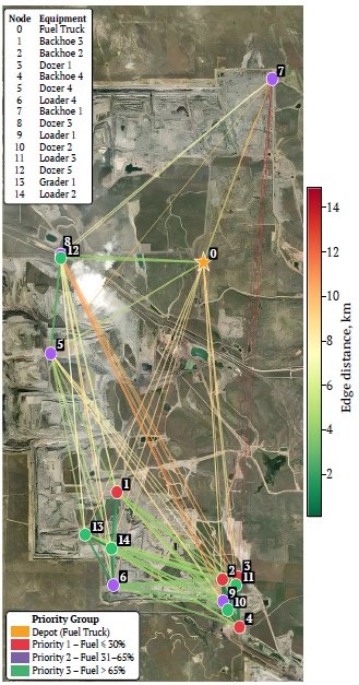
Fig. 1. Equipment locations and possible paths between equipment
To address the fuel truck routing problem, three methods are employed: Brute Force, Branch and Bound (B & B), and Ant Colony Optimization (ACO). Each method approaches the problem differently, balancing computational efficiency and solution quality while ensuring higher-priority nodes are visited first to prevent downtime, with distances based on the distance matrix in Table 2.
According to [16], the naive solution, also known as the brute-force algorithm, exhaustively calculates all possible permutations and determines the shortest length among them. Calculating and comparing all possibilities yields O(n!) time complexity for the asymmetric VRP. The sub network of first priority is considered, illustrated in Fig. 2, with distance matrix given in Table 3. If the starting vertex is node 0, then all possible paths can be calculated using Eq. 2:
P(n, r) = n!/(n − r)!, (2)
where n is number of nodes; r is number of items being arranged in a specific order.

Fig. 2. Example network (First priority group + fuel truck, given in Table 1)
Table 3
Distance submatrix for First priority group
| 0 (Depot) | 1 (Backhoe 3) | 2 (Backhoe 2) | 3 (Dozer 1) | 4 (Backhoe 4) | |
| 0 (Depot) | ∞ | 10.53 | 12.27 | 12.21 | 13.56 |
| 1 (Backhoe 3) | 10.53 | ∞ | 3.98 | 4.33 | 5.22 |
| 2 (Backhoe 2) | 12.27 | 3.98 | ∞ | 0.47 | 1.4 |
| 3 (Dozer 1) | 12.21 | 4.33 | 0.47 | ∞ | 1.35 |
| 4 (Backhoe 4) | 13.56 | 5.22 | 1.40 | 1.35 | ∞ |
Table 4
Possible permutations and distance calculations
| Number | Path | Distance | Number | Path | Distance |
| 1 | [0, 1, 2, 3, 4] | 12.57 | 13 | [0, 3, 1, 2, 4] | 18.32 |
| 2 | [0, 1, 2, 4, 3] | 13.5 | 14 | [0, 3, 1, 4, 2] | 19.56 |
| 3 | [0, 1, 3, 2, 4] | 12.97 | 15 | [0, 3, 2, 1, 4] | 18.28 |
| 4 | [0, 1, 3, 4, 2] | 13.85 | 16 | [0, 3, 2, 4, 1] | 15.70 |
| 5 | [0, 1, 4, 2, 3] | 13.85 | 17 | [0, 3, 4, 1, 2] | 19.16 |
| 6 | [0, 1, 4, 3, 2] | 13.81 | 18 | [0, 3, 4, 2, 1] | 15.35 |
| 7 | [0, 2, 1, 3, 4] | 18.29 | 19 | [0, 4, 1, 2, 3] | 19.63 |
| 8 | [0, 2, 1, 4, 3] | 19.18 | 20 | [0, 4, 1, 3, 2] | 19.98 |
| 9 | [0, 2, 3, 1, 4] | 18.64 | 21 | [0, 4, 2, 1, 3] | 19.67 |
| 10 | [0, 2, 3, 4, 1] | 15.67 | 22 | [0, 4, 2, 3, 1] | 16.17 |
| 11 | [0, 2, 4, 1, 3] | 19.57 | 23 | [0, 4, 3, 1, 2] | 19.63 |
| 12 | [0, 2, 4, 3, 1] | 15.71 | 24 | [0, 4, 3, 2, 1] | 15.77 |
Given the relatively small number of nodes in this scenario, it is feasible to evaluate all possible combinations manually or with simple computational methods. However, as the number of nodes increases, the number of potential path configurations grows exponentially, making manual computation impractical and inefficient. All possible paths and their lengths are given in Table 4 and the optimal path identified as 0–1–2–3–4 with a total distance of 12.57 km.
The Branch and Bound (B & B) algorithm [17] explores the solution space by systematically partitioning it into subproblems (branching) and computing lower bounds to prune unpromising branches (bounding). For the fuel truck routing problem, a depth-biased B & B formulation is applied using matrix reduction to efficiently prune the search space [18]. Two critical adaptations are introduced to handle the priority-constrained structure of the problem:
1) the distance matrix is defined separately for each priority group, with the ending node of one group serving as the starting node of the next
2) a dummy node with a prohibitively high traversal distance (100,000 km) to the depot is appended to each group’s subproblem, preventing the algorithm from computing a premature return to the depot between priority groups. This dummy distance is subtracted from the final solution to recover the true path length.
For each priority group, the algorithm begins by constructing a submatrix of inter-node distances, setting diagonal entries to infinity to prohibit self-loops. The matrix is then reduced by subtracting the minimum value from each row, then the minimum value from each remaining column. The sum of all subtracted minima constitutes the initial lower bound γ, representing the minimum possible distance to complete a route through all nodes in that group. This approach applied to the same priority group used in the Brute Force application. Table 5 shows the initial version of the augmented matrix.
Row reduction subtracts the row minima {10.53, 3.98, 0.47, 0.47, 1.35, 0} km, contributing γrow = 16.8 km. Column reduction subtracts the column minima {0, 0, 0, 0, 0.88, 99,989.47} km, contributing γcol = 99,990.35 km.
The raw lower bound is: 16.8 + 99,990.35 = 100,007.15 km. The 100,000 km contribution comes entirely from the Dummy column and is subtracted at the end to recover the true routing distance. The effective routing lower bound is therefore 7.15 km. The reduced version of the distance matrix is given in Table 6.
Table 5
Augmented distance submatrix for First priority group
| 0 (Depot) | 1 (Backhoe 3) | 2 (Backhoe 2) | 3 (Dozer 1) | 4 (Backhoe 4) | 5 (Dummy) | |
| 0 (Depot) | ∞ | 10.53 | 12.27 | 12.21 | 13.56 | 100,000 |
| 1 (Backhoe 3) | 10.53 | ∞ | 3.98 | 4.33 | 5.22 | 100,000 |
| 2 (Backhoe 2) | 12.27 | 3.98 | ∞ | 0.47 | 1.4 | 100,000 |
| 3 (Dozer 1) | 12.21 | 4.33 | 0.47 | ∞ | 1.35 | 100,000 |
| 4 (Backhoe 4) | 13.56 | 5.22 | 1.40 | 1.35 | ∞ | 100,000 |
| 5 (Dummy) | 0 | 100,000 | 100,000 | 100,000 | 100,000 | ∞ |
Table 6
Reduced matrix after row and column reduction (γraw = 100,007.15 km)
| 0 (Depot) | 1 (Backhoe 3) | 2 (Backhoe 2) | 3 (Dozer 1) | 4 (Backhoe 4) | 5 (Dummy) | |
| 0 (Depot) | ∞ | 0 | 1.74 | 1.68 | 2.15 | 0 |
| 1 (Backhoe 3) | 6.55 | ∞ | 0 | 0.35 | 0.36 | 6.55 |
| 2 (Backhoe 2) | 11.80 | 3.51 | ∞ | 0 | 0.043 | 10.06 |
| 3 (Dozer 1) | 11.75 | 3.86 | 0 | ∞ | 0 | 10.06 |
| 4 (Backhoe 4) | 12.21 | 3.86 | 0.043 | 0 | ∞ | 9.18 |
| 5 (Dummy) | ∞ | 0 | 100,000 | 100,000 | 100,000 | 99,999.11 |
Table 7
Branching from the Depot (Node 0)
| Branch | c(0, n) | γraw | Δγ | Total distance | Effective (−100,000) |
| 0 → Node 1 (Backhoe 3) | 0.000 | 100,007.15 | 6.55 | 100,013.71 | 13.71 km |
| 0 → Node 2 (Backhoe 2) | 1.74 | 100,007.15 | 10.06 | 100,018.95 | 18.95 km |
| 0 → Node 3 (Dozer 1) | 1.68 | 100,007.15 | 10.10 | 100,018.93 | 18.93 km |
| 0 → Node 4 (Backhoe 4) | 2.15 | 100,007.15 | 10.06 | 100,019.36 | 19.36 km |
For each candidate next node j, the branch length is computed using (Eq. 3):
c = c(0, n) + γ + Δγ, (3)
where c(0, n) is the reduced edge distance, γ = 7.15 km is the current lower bound, and Δγ is the additional reduction required after setting row 0, column j, and the back-edge j → 0 to infinity (enforcing that the depot is not revisited prematurely). The computed branch lengths are given in Table 7.
Node 1 (Backhoe 3) is selected as the first visit, having the minimum branch length of 13.71 km. The algorithm proceeds iteratively in the same fashion, updating the reduced matrix, computing branch lengths for all remaining candidates, and always selecting the node with the lowest distance, until all nodes in the First priority group are visited. The optimal sub-route for this group is completed, and the last visited node becomes the starting point for the Second priority group, which undergoes an identical matrix reduction and branching process. This continues through the Third priority group, after which the dummy node distance is subtracted to yield the true total path length.
ACO is a nature-inspired metaheuristic based on the foraging behavior of ants, introduced by [19]. It has since been widely applied to combinatorial optimization problems including the Traveling Salesman Problem, vehicle routing, and scheduling. The implementation used in this study applies ACO independently to each priority group in sequence consistent with the B & B and Brute Force formulations, with the last node of each group's optimal sub-route becoming the starting node for the next group. This ensures that priority constraints are strictly enforced: all First-priority equipment (fuel < 30%) is visited before any Second-priority equipment, and so on.
The fixed depot (Node 0, coordinates 43.721°N, –105.278°W) serves as the mandatory starting point for the First priority group. Within each group, ants construct routes by selecting nodes probabilistically according to Eq. 4:

where τij is the pheromone level on edge (i, j); ηij = 1/dij is the heuristic value (inverse of distance), α controls pheromone influence, and β controls heuristic influence. Nodes outside the current priority group are excluded from the unvisited set, ensuring the algorithm cannot cross group boundaries during route construction.
ACO parameters were determined through a systematic grid search over the primary dataset. The search space covered: iterations ∈ {50, 100}, number of ants m ∈ {5, 10, 15}, evaporation rate ρ ∈ {0.2, …, 0.9}, α ∈ {0.1, …, 1.0}, and β ∈ {0.1, …, 1.0}. The parameter combination that produced the reported result is summarized in Table 8. The pheromone deposit quantity Q is set to 1/solution_distance, so ants that find shorter routes deposit proportionally more pheromone, reinforcing better solutions over iterations.
Table 8
ACO parameter values used in the experiment
| Parameter | Symbol | Value |
| Pheromone influence | α | 0.2 |
| Heuristic influence | β | 0.8 |
| Evaporation rate | ρ | 0.2 |
| Number of ants | m | 5 |
| Number of iterations | – | 50 |
| Pheromone deposit | Q | 1/solution_distance |
| Initial pheromone | τ0 | 1 (uniform) |
The relatively low α (0.2) and high β (0.8) reflect that, in this problem, proximity is a stronger guide than historical pheromone, a sensible choice given that equipment locations change between routing decisions, and pheromone history from a previous run may not reflect the current spatial configuration. The evaporation rate of ρ = 0.2 allows pheromone trails to persist across iterations, providing sufficient memory while preventing premature convergence to suboptimal routes.
All three methods are applied to both the primary and supplementary datasets to solve the fuel truck routing problem, optimizing routes while adhering to priority constraints. The results, detailed in the subsequent section, compare their performance in terms of route distance, computation time, and scalability across the two datasets.
The first application was applied to the primary dataset of 14 equipment units to evaluate the three algorithms in terms of solution optimality, and the results are given in Table 9.
Table 9
Final path obtained by each algorithm
| Algorithm | Path length, km | Path | Optimality | Difference, % | Runtime, s |
| Brute Force | 54.39 | [0, 1, 2, 3, 4, 9, 6, 5, 7, 8, 12, 13, 14, 10, 11] | Optimal | – | 1.68 |
| Branch & Bound | 55.01 | [0, 1, 2, 3, 4, 9, 6, 5, 8, 7, 12, 13, 14, 10, 11] | Near-Optimal | 1.13 | 1.41 |
| ACO | 55.01 | [0, 1, 2, 3, 4, 9, 6, 5, 8, 7, 12, 13, 14, 10, 11] | Heuristic | 1.13 | 0.22 |
Each algorithm successfully respected the priority constraint, illustrated in Fig. 3, visiting first priority equipment before second priority and third priority in every case. The Brute Force algorithm, by exhaustively evaluating all 345,600 permutations generated across the three fixed priority groups, returned the globally optimal path. Despite its conceptual simplicity, it achieved the lowest total distance of any method, confirming its role as the ground truth benchmark against which the other algorithms are evaluated. The B & B algorithm returned a near-optimal solution with a marginally longer path, achieved through a depth-biased matrix reduction strategy that significantly reduced the number of candidate evaluations compared to Brute Force.
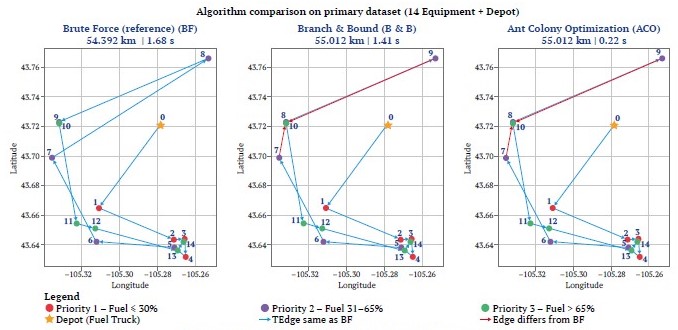
Fig. 3. Path difference between BF, B & B and ACO algorithms
The different path occurred within the Second priority group, where B & B visits Dozer 3 (Node 8) before Backhoe 1 (Node 7), while Brute Force identifies the reverse ordering as globally optimal. The total cost difference between these two orderings is 0.621 km. The mechanism behind this discrepancy is a structural property of the depth-biased matrix reduction at the heart of the B & B implementation. During the branching step within the Second priority group, Nodes 7 and 8 are geographically close to each other, with a direct inter-node distance of 7.94 km and a distance to the depot of 1.70 km and 6.32 km, respectively. When the algorithm evaluates candidate branches from their mutual predecessor node, the additional reduction term Δγ associated with selecting Node 8 first is marginally smaller than that of selecting Node 7 first. This margin arises because the matrix reduction absorbs the near-equal pairwise distances between these two nodes and the remaining unvisited candidates in slightly different proportions depending on which column is masked. The algorithm commits to Node 8 at that branching step because the computed lower-bound distance is lower, without any lookahead to evaluate whether this choice leads to a worse outcome downstream.
This behavior is a well-documented limitation of greedy depth-biased B & B implementations applied to near-equal-distance decision nodes. When two candidate branches have reduced-matrix branch lengths within a very narrow margin, the algorithm’s deterministic selection can commit to a locally plausible but globally suboptimal sequence. Brute Force avoids this entirely by evaluating all permutations explicitly.
The ACO algorithm operating through stochastic pheromone-guided construction over 50 iterations independently converged to the same path as B & B on this dataset, demonstrating that the metaheuristic exploration was sufficient to find an equally competitive solution. These results establish the baseline for the scalability analysis that follows.
In large-scale open-pit mining operations, high number of equipment units required to meet production demands poses significant challenges to the scalability of optimization algorithms. This section evaluates the computational performance of BF, B & B, and ACO algorithms, focusing on their efficiency in terms of computation time and path length as the number of equipment units increases. The scalability analysis was conducted in two parts. The first part examined the performance of all three algorithms for equipment counts ranging from 15 to 20 units, and is presented in Fig. 4. The second part extended the analysis to 38 equipment units, comparing B & B and ACO only, as Brute Force becomes computationally infeasible beyond approximately 17 nodes, and is presented in Fig. 5.
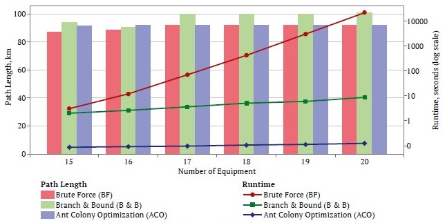
Fig. 4. Scalability analysis of Brute Force, B & B, and ACO for equipment counts up to 20
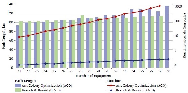
Fig. 5. Scalability analysis of B & B and ACO for equipment counts up to 38
Fig. 5 reveals a clear divergence in runtime behaviour as the number of equipment grows. Brute Force runtime grows factorially, surpassing 100 seconds at 17 nodes and reaching over 400 seconds at 17 nodes with an unequal priority group distribution. This growth rate makes real-time deployment entirely infeasible beyond this threshold. B & B demonstrates substantially better scaling behaviour within 10 to 20 equipment units range, with runtimes remaining below 15 seconds, though its growth trend is already noticeably superlinear. ACO maintains consistently sub-second runtimes across the entire range, remaining below 0.5 seconds at 20 equipment units. In terms of solution quality, Brute Force and ACO produce comparable path lengths across the tested range, while B & B occasionally yields slightly longer routes, reflecting the distances in its deterministic pruning decisions in near-equal-distance scenarios.
Fig. 6 illustrates the divergence between B & B and ACO at larger operational scales. B & B runtime grows steeply beyond 28 equipment units, exceeding 100 seconds at 29 units and becoming impractical for real-time use beyond that point. This growth pattern, driven by the combinatorial branching structure of the algorithm, makes B & B unsuitable for mines with large active fleets. ACO, by contrast, scales with near-linear runtime growth, still being under 1 second at the maximum tested scale of 38 equipment units. This result directly motivates the use of metaheuristic methods in large-scale fuel routing problems: the combination of near-optimal solution quality and manageable computation time makes ACO the only candidate among the three evaluated methods that can realistically support real-time operational decision-making at mine scale.
The present work establishes concrete and reproducible empirical thresholds: Brute Force becomes infeasible beyond approximately 17 equipment units, and B & B beyond approximately 20 units, while ACO remains computationally viable at the full tested scale of 38 units with a runtime under 1 second. These thresholds provide directly actionable guidance for practitioners and fleet management system developers. A mine operating a fleet of fewer than 17 active equipment units per routing cycle may find Brute Force sufficient for obtaining guaranteed optimal routes. A mine in the 17 to 20 units range may employ B & B as a computationally tractable exact-adjacent approach. Any mine operating beyond 20 active units that is characteristic of the large majority of modern open-pit coal and metal mines, should adopt ACO or a comparable metaheuristic as the default routing strategy. The demonstration that ACO consistently delivers near-optimal paths within 2 seconds across all tested scales provides an empirical foundation for this recommendation that was previously absent from the mining-specific routing literature.
Beyond the algorithmic benchmarking, the study highlights a broader point about optimisation in mining industry: the sustainability gains from routing efficiency are not confined to the visible paths/costs of a fuel truck itself. Optimised refueling sequences increase equipment availability, reduce the frequency of unplanned stoppages caused by fuel depletion, and allow the production cycle to run with fewer interruptions. In an industry where the capital costs of large equipment and the consequences of unplanned downtime are both substantial, even marginal improvements in routing efficiency, when applied consistently across every shift of a multi-year mine life, can accumulate into meaningful reductions in operating costs and improvements in equipment utilisation rates.
The 1.13% deviation of B & B and ACO from the Brute Force optimum must be evaluated against the correct reference point, which is not perfection, but the realistic alternative of unoptimized routing. In a mining operation without a systematic routing algorithm, a fuel truck operator follows an ad hoc sequence based on proximity estimation or personal judgment, which is effectively a random permutation of equipment visits within each priority group. To quantify what this means concretely, all 24 possible orderings of the First priority group (four equipment units with fuel levels below 30%) were evaluated against the 14-equipment unit primary dataset. The optimal routing for this group alone amounts to 16.33 km. A randomly selected ordering route distance averages 20.51 km, representing a 25.6% excess over optimal, and in the worst case reaches 23.57 km, a 44.4% excess. The 1.13% gap between ACO and Brute Force is therefore not a disadvantage of ACO, but, on contrary, a demonstration that metaheuristic optimization delivers near-perfect efficiency relative to the realistic operational baseline. This perspective becomes particularly important when considering the scale of real open-pit mining operations. Medium to large mine sites routinely operate fleets of 100 to 150 active equipment units per shift, with fuel levels changing continuously throughout the day. At these scales, Brute Force is not merely slow but categorically infeasible: the number of permutations to evaluate grows factorially and exceeds any practical computational limits by orders of magnitude. B & B, as demonstrated by the scalability results in this study, becomes impractical beyond approximately 20 equipment units. For a mine with 100 to 150 units, the choice is not between an exact algorithm and ACO, it is between ACO and no algorithm at all. Accepting a sub-2% deviation from the theoretical optimum in exchange for a routing solution computed in under two seconds is not a limitation of the metaheuristic approach, it is the only operationally viable path forward. The scalability data confirm this: ACO’s runtime at 38 equipment units is 1.59 seconds, and its near-linear growth trend indicates that even at 100 units the computation would remain well within the time constraints of a real-time routing system.
The contribution of this study is the systematic empirical characterisation of three algorithmically distinct classes of methods, namely an exact method (BF), a bounded exact method (B & B), and a metaheuristic (ACO), applied to a problem formulation that has not been previously addressed in the literature: priority-constrained fuel truck routing in open-pit mining where priorities are defined by real-time fuel levels rather than static demand parameters.
This distinction carries genuine practical weight. Because priority groups are determined by the instantaneous fuel tankage of each piece of equipment at the moment a routing decision is made, they cannot be pre-computed, approximated from historical patterns, or treated as fixed. A routing algorithm that performs well on a static priority assignment may behave very differently when group membership shifts between cycles, as it does in real operations. No prior study has benchmarked the scalability limits of these three algorithm classes under this specific constraint.
The present study operates under several simplifying assumptions that should be presented. First, only a single fuel truck was modelled. In practice, large open-pit mines typically deploy two or more fuel trucks operating simultaneously that introduces coordination and scheduling complexity that is absent from the current formulation. Extending the model to multi-truck scenarios would require addressing vehicle-to-vehicle task allocation, potential route conflicts on shared haul roads, and the synchronisation of refueling completion times. Second, the depot location is treated as fixed and stationary. In reality, the fuel truck's base position may change between shifts or it may itself be a mobile unit that would alter the initial distance matrix at each routing cycle. Third, the geodesic distance measure used throughout this study assumes free-space travel between nodes, ignoring the actual road network, road grades, and directional constraints of the mine layout. Real haul road distances can differ substantially from geodesic distances, particularly in mines with complex ramp and bench geometries. Fourth, the model assumes that fuel demand is known and static at the moment of routing. Dynamic changes in fuel consumption rate during the cycle are not accounted for.
Future work could address each of these limitations in turn. The extension to multiple fuel trucks represents the most immediate and impactful line of inquiry, as it better reflects operational reality and introduces combinatorial complexity that would
1. Liu S. Q., Kozan E. New graph-based algorithms to efficiently solve large scale open pit mining optimisation problems. Expert Systems with Applications. 2016;23(C):59–65. https://doi.org/10.1016/j.eswa.2015.08.044
2. Hasozdemir K., Erçelebi S. Enhancing the performance of integer models for addressing the long-term production planning problem in open pit mines by decision variable fixation based on parametric analysis of the final pit limit. Mining Science and Technology (Russia). 2024;9(2):74-84. https://doi.org/10.17073/2500-0632-2023-09-156
3. Pham V. H. S., Nguyen V. N. Cement transport vehicle routing with a hybrid sine cosine optimization algorithm. Advances in Civil Engineering. 2023;2023:2728039. https://doi.org/10.1155/2023/2728039
4. Dereci U., Karabekmez M. E. The applications of multiple route optimization heuristics and meta-heuristic algorithms to solid waste transportation: A case study in Turkey. Decision Analytics Journal. 2022;4:100113. https://doi.org/10.1016/j.dajour.2022.100113
5. Khajouei M. H. S. H., Lotfi M., Ebrahimi A., Jafari S. Water truck routing optimization in open pit mines using the general algebraic modelling system approach. In: Molamohamadi Z., Babaee Tirkolaee E., Mirzazadeh A., Weber G.W. (Eds.) Logistics and Supply Chain Management. LSCM 2020. Communications in Computer and Information Science. Vol. 1458. Cham: Springer; 2021. Pp. 84–98. https://doi.org/10.1007/978-3-030-89743-7_14
6. Solid K., Komarudin. Water truck routing and scheduling optimization in mining operations with inventory function based on mixed integer linear programming. In: ICIDE 2017. Proceedings of the 2017 International Conference on Industrial Design Engineering. Pp. 127–132. https://doi.org/10.1145/3178264.3178288
7. Yaping Q., Bossman M. Logistics and supply chain management efficiency strategy for ghana’s mining industry. European Journal of Business and Management Research. 2021;6(2). https://doi.org/10.24018/ejbmr.2021.6.2.779
8. Wang L., Kinable J., van Woensel T. The fuel replenishment problem: A split-delivery multi-compartment vehicle routing problem with multiple trips. Computers & Operations Research. 2020;118:104904. https://doi.org/10.1016/j.cor.2020.104904
9. Freitas M., Silva J. M. P., Uchoa E. A unified exact approach for Clustered and Generalized Vehicle Routing Problems. Computers & Operations Research. 2023;149:106040. https://doi.org/10.1016/j.cor.2022.106040
10. Ribeiro R. G., Junior J. R. C., Cota L. P. et al. Unmanned aerial vehicle location routing problem with charging stations for belt conveyor inspection system in the mining industry. In: IEEE Transactions on Intelligent Transportation Systems. 2020;21(10):4186–4195. https://doi.org/10.1109/TITS.2019.2939094
11. Wang A., Subramanyam A., Gounaris C. E. Robust vehicle routing under uncertainty via branch-price-and-cut. Optimization and Engineering. 2022;23(4):1895–1948. https://doi.org/10.1007/s11081-021-09680-6
12. Liu G., Chai S., Bai R. et al. Route selection algorithm of open-pit mine transportation system. Meitan Xuebao/Journal of the China Coal Society. 2019;44(12). (In Chinese) https://doi.org/10.13225/j.cnki.jccs.2017.0308
13. Andreica M. I., Briciu S., Andreica M. E. Algorithmic solutions to some transportation optimization problems with applications in the metallurgical. Metalurgia International. 2009;14(Spec. Iss. 5):46–53. URL: https://hal.science/hal-00472811v1
14. Rizzoli A. E., Montemanni R., Lucibello E., Gambardella L. M. Ant colony optimization for real-world vehicle routing problems. Swarm Intelligence. 2007;1(2):135–151. https://doi.org/10.1007/s11721-007-0005-x
15. Baskar A. Simple single and multi-facility location models using great circle distance. In: ITM Web of Conferences. 2021;37:01001. https://doi.org/10.1051/itmconf/20213701001
16. Goyal S. A survey on travelling salesman problem. In: Midwest Instruction and Computing Symposium (MICS). 2010. URL: https://www.micsymposium.org/mics_2010_proceedings/mics2010_submission_51.pdf
17. Applegate D. L., Bixby R. E., Chvátal V., Cook W. J. The traveling salesman problem: A computational study. 2011. 608 p.
18. Jünger M., Reinelt G., Rinaldi G. Chapter 4 The traveling salesman problem. In: Ball M. O., Magnanti T. L., Monma C. L., Nemhauser G. L. (Eds.) Handbooks in Operations Research and Management Science. Vol 7. Network Models. Amsterdam: Elsevier Science B.V.; 1995. Pp. 225–330.
19. Dorigo M., Maniezzo V., Colorni A. Ant system: optimization by a colony of cooperating agents. In: IEEE Transactions on Systems, Man, and Cybernetics, Part B: Cybernetics. 1996;26(1):1–13.
Kursat Hasozdemir – PhD, Research Assistant, Department of Mining Engineering
Istanbul
Scopus ID 57211503596
Muhammet Mustafa Kahraman – PhD, Associate Professor, Department of Mining Engineering
Istanbul
Scopus ID 55366162500
Özge Ece Özalp – PhD‑Student, Research and Teaching Assistant, Department of Mining Engineering,
Istanbul
Hasozdemir K., Kahraman M.M., Özalp Ö.E. Comparison of travel route optimization algorithms performance for fuel truck routing problem in open pit mines. Mining Science and Technology (Russia). https://doi.org/10.17073/2500-0632-2025-05-965




Editor-in-Chief
Petrov V.L. Email this article (Login required)
Email the author (Login required)
Email this article (Login required)
Email the author (Login required) 119049, Moscow, Leninsky Prospect, 4, b. 1
The National University of Science and Technology MISIS (NUST MISIS)
Tel.: +7 (968) 848-61-24
E-mail: send@misis.ru